실습 10: 텍스트를 숫자로 — 토큰화와 임베딩

Open In Colab

시나리오 — 오늘 만들 것

무대를 또 한 번 바꾼다. 입력이 한국어 문장이다.

\[\text{"이 영화 진짜 재밌다"} \;\to\; \text{토큰} \;\to\; \text{번호} \;\to\; (B, T) \;\to\; \text{임베딩} \;\to\; (B, T, d)\]

문장 한 줄이 텐서가 되기까지를 한 단계씩 확인한 뒤, 네이버 영화 리뷰 2만 건으로 감성 분류기를 학습시킨다. 글자를 숫자로 바꾸는 것만 새로 배우면, 학습 루프는 3주차 그대로다.

대응 이론: Ch10 텍스트를 숫자로
도구: HuggingFace 토크나이저 (klue/bert-base)
데이터: NSMC (네이버 영화 리뷰) — 실제 한국어 리뷰

이번 주에 익히는 것

개념	이론과의 대응
토큰화 · 서브워드	BPE 손계산 (Ch10)
어휘 사전 · `[UNK]`	미등록 단어 문제 (Ch10)
원-핫의 실패	내적이 항상 0 (Ch10)
`nn.Embedding`	임베딩 파라미터 \(V \times d\), 편향 없음 (Ch10)
내적 · 코사인 유사도	유사도 손계산 (Ch10)
`(B, T, d)` · 패딩 · 마스크	문장을 텐서로 (Ch10)

1. 텍스트를 조각내기

import numpy as np
import pandas as pd
import torch
import torch.nn as nn
import torch.nn.functional as F
import matplotlib.pyplot as plt

torch.manual_seed(42)

corpus = [
    "딥러닝은 데이터로 규칙을 배운다",
    "기계학습은 데이터로 규칙을 배운다",
    "딥러닝은 이미지를 잘 분류한다",
    "자동차는 도로를 달린다",
]
for s in corpus:
    print(s)

딥러닝은 데이터로 규칙을 배운다
기계학습은 데이터로 규칙을 배운다
딥러닝은 이미지를 잘 분류한다
자동차는 도로를 달린다

1-1. 무엇을 한 단위로 셀 것인가

def by_space(s):  return s.split()
def by_char(s):   return list(s.replace(' ', ''))

rows = []
for name, fn in [('공백 단위', by_space), ('글자 단위', by_char)]:
    toks = [t for s in corpus for t in fn(s)]
    rows.append({'방식': name, '전체 토큰 수': len(toks), '어휘 크기': len(set(toks))})
print(pd.DataFrame(rows).to_string(index=False))

print('\n공백 단위:', by_space(corpus[0]))
print('글자 단위:', by_char(corpus[0]))

   방식  전체 토큰 수  어휘 크기
공백 단위       15     11
글자 단위       52     32

공백 단위: ['딥러닝은', '데이터로', '규칙을', '배운다']
글자 단위: ['딥', '러', '닝', '은', '데', '이', '터', '로', '규', '칙', '을', '배', '운', '다']

두 방식의 맞바꿈

공백 단위: 시퀀스는 짧지만 어휘가 폭발한다. “배운다 / 배웠다 / 배우고”가 전부 다른 단어다.
글자 단위: 어휘는 작지만 시퀀스가 길어지고, 글자 하나에는 의미가 거의 없다.

그래서 실제로는 그 사이 — 서브워드를 쓴다.

1-2. BPE를 직접 구현 — Ch10의 손계산 재현

장난감 문자열 aaabdaaabac 에 병합을 3번 적용한다.

from collections import Counter

def most_frequent_pair(tokens, order):
    """최다 빈도 쌍. 동률이면 어휘에 먼저 들어온 기호를 우선한다."""
    pairs = Counter(zip(tokens[:-1], tokens[1:]))
    if not pairs:
        return None, 0
    best = max(pairs.items(),
               key=lambda kv: (kv[1], -order[kv[0][0]], -order[kv[0][1]]))
    return best

def merge(tokens, pair, new_symbol):
    out, i = [], 0
    while i < len(tokens):
        if i < len(tokens)-1 and (tokens[i], tokens[i+1]) == pair:
            out.append(new_symbol); i += 2
        else:
            out.append(tokens[i]); i += 1
    return out

tokens = list('aaabdaaabac')
order = {c: i for i, c in enumerate(sorted(set(tokens)))}   # 어휘 진입 순서
rows = [{'단계': 0, '토큰열': ' '.join(tokens), '토큰 수': len(tokens),
         '최다 빈도 쌍': f'{most_frequent_pair(tokens, order)[0]} — {most_frequent_pair(tokens, order)[1]}회',
         '병합': ''}]

for step, sym in enumerate(['Z', 'Y', 'X'], start=1):
    pair, cnt = most_frequent_pair(tokens, order)
    tokens = merge(tokens, pair, sym)
    order[sym] = len(order)                                 # 새 기호는 맨 뒤에 추가
    nxt, ncnt = most_frequent_pair(tokens, order)
    rows.append({'단계': step, '토큰열': ' '.join(tokens), '토큰 수': len(tokens),
                 '최다 빈도 쌍': f'{nxt} — {ncnt}회',
                 '병합': f'{"".join(pair)} → {sym}'})

print(pd.DataFrame(rows).to_string(index=False))
print('\n어휘 사전:', list(order.keys()))

 단계                   토큰열  토큰 수         최다 빈도 쌍     병합
  0 a a a b d a a a b a c    11 ('a', 'a') — 4회       
  1     Z a b d Z a b a c     9 ('a', 'b') — 2회 aa → Z
  2         Z Y d Z Y a c     7 ('Z', 'Y') — 2회 ab → Y
  3             X d X a c     5 ('a', 'c') — 1회 ZY → X

어휘 사전: ['a', 'b', 'c', 'd', 'Z', 'Y', 'X']

토큰 수는 11 → 5로 줄고, 어휘는 4개 → 7개로 늘었다. 자주 나오는 조각을 하나의 토큰으로 승격시키는 것이 BPE의 전부다.

단계 1에서 (Z, a) 와 (a, b) 가 둘 다 2회로 동률이다. 동률일 때 무엇을 고를지는 미리 정해 두어야 결과가 재현된다 — 여기서는 어휘에 먼저 들어온 기호를 우선하는 규칙을 썼다. 실제 토크나이저도 이런 규칙을 학습 시점에 고정해 두고 파일로 저장한다.

1-3. 실제 토크나이저

from transformers import AutoTokenizer

tok = AutoTokenizer.from_pretrained('klue/bert-base')
print('토크나이저 :', type(tok).__name__)
print('어휘 크기  :', tok.vocab_size)
print('특수 토큰  :', {'[PAD]': tok.pad_token_id, '[UNK]': tok.unk_token_id,
                       '[CLS]': tok.cls_token_id, '[SEP]': tok.sep_token_id})

토크나이저 : BertTokenizerFast
어휘 크기  : 32000
특수 토큰  : {'[PAD]': 0, '[UNK]': 1, '[CLS]': 2, '[SEP]': 3}

for s in ['딥러닝은 즐겁다', '기계학습은 어렵다', 'Deep learning is fun', '췩췩폭폭']:
    print(f'{s:22s} → {tok.tokenize(s)}')

딥러닝은 즐겁다               → ['딥', '##러', '##닝', '##은', '즐겁', '##다']
기계학습은 어렵다              → ['기계', '##학습', '##은', '어렵', '##다']
Deep learning is fun   → ['De', '##ep', 'le', '##ar', '##ning', 'is', 'f', '##un']
췩췩폭폭                   → ['[UNK]']

## 는 앞 토큰에 이어 붙는 조각이라는 표시다. 자주 쓰이는 말은 통째로, 드문 말은 잘게 쪼개진다 — 데이터의 빈도가 그대로 칼자국이 되었다.

직접 해보기 ① — 내 문장은 몇 조각이 되는가

자기 이름과 좋아하는 음식이 들어간 문장을 토큰화해 보시오. 몇 조각으로 쪼개지는가? 통째로 남는 말과 잘게 쪼개지는 말의 차이는 무엇인가?

my_sentence = None            # ← 문장을 적으세요

print(tok.tokenize(my_sentence))
print('토큰 수:', len(tok.tokenize(my_sentence)), ' / 글자 수:', len(my_sentence))

예시 보기

for s_ in ['오늘 점심은 김치찌개를 먹었다', '부경대학교 시스템경영공학부', '뮐러리어착시']:
    t_ = tok.tokenize(s_)
    print(f'{s_:22s} → {len(t_):2d}조각  {t_}')

오늘 점심은 김치찌개를 먹었다       →  8조각  ['오늘', '점심', '##은', '김치찌개', '##를', '먹', '##었', '##다']
부경대학교 시스템경영공학부         →  8조각  ['부경', '##대', '##학교', '시스템', '##경영', '##공', '##학', '##부']
뮐러리어착시                 →  1조각  ['[UNK]']

enc = tok('딥러닝은 즐겁다')
print('input_ids     :', enc['input_ids'])
print('attention_mask:', enc['attention_mask'])
print('되돌리기      :', tok.convert_ids_to_tokens(enc['input_ids']))
print('문자열로      :', tok.decode(enc['input_ids']))

input_ids     : [2, 893, 2030, 2944, 2073, 7455, 2062, 3]
attention_mask: [1, 1, 1, 1, 1, 1, 1, 1]
되돌리기      : ['[CLS]', '딥', '##러', '##닝', '##은', '즐겁', '##다', '[SEP]']
문자열로      : [CLS] 딥러닝은 즐겁다 [SEP]

앞뒤에 [CLS], [SEP] 가 자동으로 붙었다. 모델마다 요구하는 특수 토큰이 다르므로 토크나이저와 모델은 반드시 짝을 맞춰야 한다.

2. 어휘 사전 만들기

토크나이저가 하는 일을 작은 규모로 직접 해 본다.

tokens_all = sorted({t for s in corpus for t in by_space(s)})
stoi = {'[PAD]': 0, '[UNK]': 1}
for t in tokens_all:
    stoi[t] = len(stoi)
itos = {i: s for s, i in stoi.items()}

print('어휘 크기 V :', len(stoi))
print(stoi)

어휘 크기 V : 13
{'[PAD]': 0, '[UNK]': 1, '규칙을': 2, '기계학습은': 3, '달린다': 4, '데이터로': 5, '도로를': 6, '딥러닝은': 7, '배운다': 8, '분류한다': 9, '이미지를': 10, '자동차는': 11, '잘': 12}

def encode(s):
    return [stoi.get(t, stoi['[UNK]']) for t in by_space(s)]

def decode(ids):
    return ' '.join(itos[i] for i in ids)

ids = encode(corpus[0])
print('원문   :', corpus[0])
print('인덱스 :', ids)
print('복원   :', decode(ids))
print('\n처음 보는 단어:', encode('로봇은 걷는다'), '← 둘 다 [UNK](1)')

원문   : 딥러닝은 데이터로 규칙을 배운다
인덱스 : [7, 5, 2, 8]
복원   : 딥러닝은 데이터로 규칙을 배운다

처음 보는 단어: [1, 1] ← 둘 다 [UNK](1)

3. 원-핫으로는 왜 안 되는가

V = len(stoi)
def onehot(i):
    v = torch.zeros(V); v[i] = 1.0; return v

a, b, c = onehot(stoi['딥러닝은']), onehot(stoi['기계학습은']), onehot(stoi['자동차는'])
print('딥러닝은 · 기계학습은 =', float(a @ b))
print('딥러닝은 · 자동차는   =', float(a @ c))
print('딥러닝은 · 딥러닝은   =', float(a @ a))

딥러닝은 · 기계학습은 = 0.0
딥러닝은 · 자동차는   = 0.0
딥러닝은 · 딥러닝은   = 1.0

서로 다른 단어는 무조건 내적이 0이다. “딥러닝”과 “기계학습”이 가까운지, “자동차”와 먼지를 원-핫은 표현할 방법이 없다.

rows = []
for V_ in [len(stoi), 5_000, 32_000, 50_257]:
    rows.append({'어휘 V': f'{V_:,}', '원-핫 한 단어의 크기': f'{V_:,} 차원',
                 '0이 아닌 값': 1, '메모리(float32)': f'{V_*4/1024:.1f} KB'})
print(pd.DataFrame(rows).to_string(index=False))

  어휘 V 원-핫 한 단어의 크기  0이 아닌 값 메모리(float32)
    13        13 차원        1       0.1 KB
 5,000     5,000 차원        1      19.5 KB
32,000    32,000 차원        1     125.0 KB
50,257    50,257 차원        1     196.3 KB

4. 임베딩 — 단어를 좌표로

4-1. `nn.Embedding` 은 표에서 행을 꺼내는 것

d = 8
emb = nn.Embedding(num_embeddings=V, embedding_dim=d)

print('가중치 shape :', tuple(emb.weight.shape), ' = (V, d)')
print('파라미터 수  :', sum(p.numel() for p in emb.parameters()), ' = V x d =', V*d)
print('편향이 있는가:', any('bias' in n for n, _ in emb.named_parameters()))

가중치 shape : (13, 8)  = (V, d)
파라미터 수  : 104  = V x d = 104
편향이 있는가: False

임베딩에는 편향이 없다

\[\text{임베딩 파라미터 수} = V \times d\]

완전연결층과 달리 곱셈이 아니라 “표에서 행을 꺼내는” 연산이기 때문이다.

i = stoi['딥러닝은']
print('emb(i)      :', emb(torch.tensor(i)).detach().numpy().round(4))
print('weight[i]   :', emb.weight[i].detach().numpy().round(4))
print('같은가      :', torch.allclose(emb(torch.tensor(i)), emb.weight[i]))

emb(i)      : [-1.4032  0.036  -0.0635  0.6756 -0.0978  1.8446 -1.1845  1.3835]
weight[i]   : [-1.4032  0.036  -0.0635  0.6756 -0.0978  1.8446 -1.1845  1.3835]
같은가      : True

# 원-핫 x 가중치 행렬 = 행 꺼내기 (수학적으로 같다)
oh = onehot(i)
print('원-핫 @ weight :', (oh @ emb.weight).detach().numpy().round(4))

원-핫 @ weight : [-1.4032  0.036  -0.0635  0.6756 -0.0978  1.8446 -1.1845  1.3835]

곱셈으로 해도 결과는 같지만, \(V\) 가 5만이면 5만 번 곱해서 1개만 남기는 낭비다. 그래서 실제로는 인덱싱으로 구현한다.

4-2. Ch10의 파라미터 표 재현

rows = []
for V_, d_, note in [(5_000, 128, ''), (32_000, 768, 'klue/bert-base 규모'),
                     (50_257, 768, 'GPT-2')]:
    rows.append({'어휘 V': f'{V_:,}', '차원 d': d_,
                 '파라미터 V x d': f'{V_*d_:,}', '비고': note})
print(pd.DataFrame(rows).to_string(index=False))

  어휘 V  차원 d 파라미터 V x d                비고
 5,000   128    640,000                  
32,000   768 24,576,000 klue/bert-base 규모
50,257   768 38,597,376             GPT-2

GPT-2는 임베딩 층 하나만으로 3,860만 파라미터다.

5. 유사도 — 내적과 코사인

5-1. Ch10의 장난감 임베딩 재현

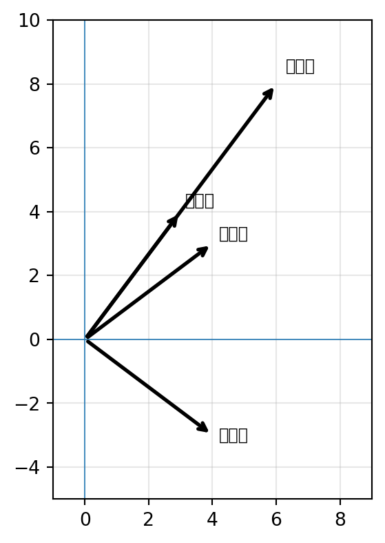
\[\text{고양이} = (3, 4), \quad \text{강아지} = (4, 3), \quad \text{호랑이} = (6, 8), \quad \text{자동차} = (4, -3)\]

vecs = {'고양이': torch.tensor([3., 4.]), '강아지': torch.tensor([4., 3.]),
        '호랑이': torch.tensor([6., 8.]), '자동차': torch.tensor([4., -3.])}

rows = []
for w1, w2 in [('고양이','강아지'), ('고양이','호랑이'), ('강아지','호랑이'),
               ('고양이','자동차'), ('강아지','자동차')]:
    a, b = vecs[w1], vecs[w2]
    dot = float(a @ b)
    na, nb = float(a.norm()), float(b.norm())
    rows.append({'쌍': f'{w1} · {w2}', '내적': dot, '|a|': round(na, 2), '|b|': round(nb, 2),
                 '코사인': round(dot/(na*nb), 4)})
print(pd.DataFrame(rows).to_string(index=False))

        쌍   내적  |a|  |b|  코사인
고양이 · 강아지 24.0  5.0  5.0 0.96
고양이 · 호랑이 50.0  5.0 10.0 1.00
강아지 · 호랑이 48.0  5.0 10.0 0.96
고양이 · 자동차  0.0  5.0  5.0 0.00
강아지 · 자동차  7.0  5.0  5.0 0.28

a, b = vecs['고양이'], vecs['강아지']
print('직접 계산 :', round(float(a @ b) / (float(a.norm()) * float(b.norm())), 6))
print('F.cosine_similarity:', round(float(F.cosine_similarity(a[None], b[None])), 6))

직접 계산 : 0.96
F.cosine_similarity: 0.96

5-2. 왜 내적이 아니라 코사인인가

print('강아지 · 호랑이 내적 :', float(vecs['강아지'] @ vecs['호랑이']))
print('고양이 · 강아지 내적 :', float(vecs['고양이'] @ vecs['강아지']))
print()
print('강아지 · 호랑이 코사인:', round(float(F.cosine_similarity(vecs['강아지'][None], vecs['호랑이'][None])), 4))
print('고양이 · 강아지 코사인:', round(float(F.cosine_similarity(vecs['고양이'][None], vecs['강아지'][None])), 4))
print('\n호랑이 벡터의 크기:', float(vecs['호랑이'].norm()), '← 다른 벡터의 두 배')

강아지 · 호랑이 내적 : 48.0
고양이 · 강아지 내적 : 24.0

강아지 · 호랑이 코사인: 0.96
고양이 · 강아지 코사인: 0.96

호랑이 벡터의 크기: 10.0 ← 다른 벡터의 두 배

내적은 방향이 같아도 벡터가 길면 커진다. 코사인은 크기를 나눠 없애므로 방향(의미)만 남는다.

fig, ax = plt.subplots(figsize=(4.6, 4.2))
for name, v in vecs.items():
    ax.annotate('', xy=v.tolist(), xytext=(0, 0),
                arrowprops=dict(arrowstyle='->', lw=2))
    ax.text(v[0]*1.05, v[1]*1.05, name, fontsize=9)
ax.set_xlim(-1, 9); ax.set_ylim(-5, 10); ax.axhline(0, lw=0.6); ax.axvline(0, lw=0.6)
ax.grid(alpha=0.3); ax.set_aspect('equal')
plt.tight_layout(); plt.show()

5-3. 모든 쌍을 한 번에

names = list(vecs.keys())
Vm = torch.stack([vecs[n] for n in names])                 # (4, 2)
Vn = Vm / Vm.norm(dim=1, keepdim=True)                     # 행마다 크기 1로
C = Vn @ Vn.T                                              # 코사인 행렬
print('shape :', tuple(C.shape))
print(pd.DataFrame(C.numpy().round(2), index=names, columns=names))

shape : (4, 4)
      고양이   강아지   호랑이   자동차
고양이  1.00  0.96  1.00 -0.00
강아지  0.96  1.00  0.96  0.28
호랑이  1.00  0.96  1.00 -0.00
자동차 -0.00  0.28 -0.00  1.00

정규화한 뒤 행렬 곱 한 번이면 모든 쌍의 코사인이 나온다. 1주차의 X @ w 와 같은 요령이다.

6. 문장을 텐서로 — `(B, T, d)`

6-1. 길이가 다른 문장을 한 배치에

batch = ['딥러닝은 즐겁다', '기계학습은 데이터로 규칙을 배운다', '좋다']
for s in batch:
    print(f'{s:24s} → {len(tok.tokenize(s))} 토큰')

딥러닝은 즐겁다                 → 6 토큰
기계학습은 데이터로 규칙을 배운다       → 8 토큰
좋다                       → 2 토큰

텐서는 직사각형이어야 한다. 패딩으로 길이를 맞춘다.

enc = tok(batch, padding=True, return_tensors='pt')
print('input_ids shape      :', tuple(enc['input_ids'].shape), ' = (B, T)')
print('attention_mask shape :', tuple(enc['attention_mask'].shape))
print()
print('input_ids:\n', enc['input_ids'].numpy())
print('\nattention_mask:\n', enc['attention_mask'].numpy())

input_ids shape      : (3, 10)  = (B, T)
attention_mask shape : (3, 10)

input_ids:
 [[    2   893  2030  2944  2073  7455  2062     3     0     0]
 [    2  5276 21468  2073  5189  2200  6094  2069 21527     3]
 [    2  1560  2062     3     0     0     0     0     0     0]]

attention_mask:
 [[1 1 1 1 1 1 1 1 0 0]
 [1 1 1 1 1 1 1 1 1 1]
 [1 1 1 1 0 0 0 0 0 0]]

for row_ids, row_mask in zip(enc['input_ids'], enc['attention_mask']):
    toks = tok.convert_ids_to_tokens(row_ids)
    print([f'{t}({m})' for t, m in zip(toks, row_mask.tolist())])

['[CLS](1)', '딥(1)', '##러(1)', '##닝(1)', '##은(1)', '즐겁(1)', '##다(1)', '[SEP](1)', '[PAD](0)', '[PAD](0)']
['[CLS](1)', '기계(1)', '##학습(1)', '##은(1)', '데이터(1)', '##로(1)', '규칙(1)', '##을(1)', '배운다(1)', '[SEP](1)']
['[CLS](1)', '좋(1)', '##다(1)', '[SEP](1)', '[PAD](0)', '[PAD](0)', '[PAD](0)', '[PAD](0)', '[PAD](0)', '[PAD](0)']

마스크의 0이 패딩 자리다. 뒤에 나올 어텐션이 이 자리를 보지 않게 만드는 데 쓰인다.

6-2. 임베딩을 통과시키면 `(B, T, d)`

d_model = 16
emb2 = nn.Embedding(tok.vocab_size, d_model, padding_idx=tok.pad_token_id)

X = emb2(enc['input_ids'])
print('input_ids :', tuple(enc['input_ids'].shape), ' (B, T)')
print('임베딩 후 :', tuple(X.shape), ' (B, T, d)')
print()
print('B = 문장 수      :', X.shape[0])
print('T = 토큰 수(패딩 포함):', X.shape[1])
print('d = 임베딩 차원  :', X.shape[2])

input_ids : (3, 10)  (B, T)
임베딩 후 : (3, 10, 16)  (B, T, d)

B = 문장 수      : 3
T = 토큰 수(패딩 포함): 10
d = 임베딩 차원  : 16

padding_idx 를 지정하면 [PAD] 의 임베딩이 0 벡터로 고정되고 학습되지도 않는다.

print('[PAD] 임베딩:', emb2.weight[tok.pad_token_id].detach().numpy().round(4))

[PAD] 임베딩: [0. 0. 0. 0. 0. 0. 0. 0. 0. 0. 0. 0. 0. 0. 0. 0.]

6-3. 마스크를 쓰지 않으면 생기는 일

문장 하나를 벡터 하나로 요약하려고 토큰 임베딩을 평균낸다고 하자.

mask = enc['attention_mask']                    # (B, T)

naive = X.mean(dim=1)                           # 패딩까지 평균에 넣는다
masked = (X * mask[:, :, None]).sum(1) / mask.sum(1, keepdim=True)

print('naive  shape:', tuple(naive.shape))
print('masked shape:', tuple(masked.shape))
print()
for i, s in enumerate(batch):
    diff = float((naive[i] - masked[i]).abs().max())
    print(f'{s:24s} 실제 토큰 {int(mask[i].sum())}/{mask.shape[1]}  최대 차이 {diff:.4f}')

naive  shape: (3, 16)
masked shape: (3, 16)

딥러닝은 즐겁다                 실제 토큰 8/10  최대 차이 0.1416
기계학습은 데이터로 규칙을 배운다       실제 토큰 10/10  최대 차이 0.0000
좋다                       실제 토큰 4/10  최대 차이 0.5263

짧은 문장일수록 패딩이 많고, 그만큼 평균이 0 쪽으로 끌려간다. (B, T, d) 를 다룰 때는 항상 마스크를 함께 들고 다녀야 한다.

직접 해보기 ② — 마스크 평균을 직접 구현하기

(B, T, d) 텐서 X 와 (B, T) 마스크 mask 를 받아 패딩을 뺀 평균 (B, d) 를 돌려주는 함수를 작성하시오.

def masked_mean(X, mask):
    return None                # ← 여기를 채우세요

got = masked_mean(X, mask)
assert got is not None and tuple(got.shape) == (3, 16), f'모양이 다릅니다: {tuple(got.shape)}'
assert torch.allclose(got, masked, atol=1e-5), '값이 다릅니다'
print('통과', tuple(got.shape))

정답 코드 보기

def masked_mean(X, mask):
    m = mask.unsqueeze(-1).float()
    return (X * m).sum(1) / m.sum(1).clamp(min=1)

print('통과', tuple(masked_mean(X, mask).shape),
      torch.allclose(masked_mean(X, mask), masked, atol=1e-5))

통과 (3, 16) True

clamp(min=1) 은 한 문장이 통째로 패딩일 때 0으로 나누는 사고를 막는다.

6.5. 완성 — 영화 리뷰 감성 분류기

지금까지 만든 조각(토큰화 → 인덱스 → 패딩 → 임베딩 → 마스크 평균)을 이어 실제 한국어 리뷰를 긍정/부정으로 분류한다.

6-5-1. 데이터 — NSMC

import time
from torch.utils.data import TensorDataset, DataLoader

TRAIN_URL = 'https://raw.githubusercontent.com/e9t/nsmc/master/ratings_train.txt'
TEST_URL  = 'https://raw.githubusercontent.com/e9t/nsmc/master/ratings_test.txt'

train_raw = pd.read_csv(TRAIN_URL, sep='\t').dropna()
test_raw  = pd.read_csv(TEST_URL,  sep='\t').dropna()

print('전체 :', len(train_raw), '/', len(test_raw))
print('라벨 :', train_raw['label'].value_counts().to_dict(), ' (1=긍정, 0=부정)')
train_raw.head(3)

전체 : 149995 / 49997
라벨 : {0: 75170, 1: 74825}  (1=긍정, 0=부정)

	id	document	label
0	9976970	아 더빙.. 진짜 짜증나네요 목소리	0
1	3819312	흠...포스터보고 초딩영화줄....오버연기조차 가볍지 않구나	1
2	10265843	너무재밓었다그래서보는것을추천한다	0

# 수업 시간 안에 끝나도록 일부만 사용한다
train_df = train_raw.sample(20000, random_state=42)
test_df  = test_raw.sample(5000,  random_state=42)

for i in range(3):
    r = train_df.iloc[i]
    print(f'[{r["label"]}] {r["document"][:60]}')

[1] 원본이 최고
[1] 스릴감과 훈훈함이 있는 영화.
[1] 굉장히 저평가되는 영화중 하나라고 생각함

6-5-2. 문장을 `(B, T)` 로

MAX_LEN = 48

def encode(df):
    e = tok(list(df['document']), padding='max_length', truncation=True,
            max_length=MAX_LEN, return_tensors='pt')
    return e['input_ids'], e['attention_mask'], torch.tensor(df['label'].to_numpy())

t0 = time.time()
Xtr, Mtr, ytr = encode(train_df)
Xte, Mte, yte = encode(test_df)
print(f'토큰화 {time.time()-t0:.1f}초')
print('입력', tuple(Xtr.shape), ' 마스크', tuple(Mtr.shape), ' 정답', tuple(ytr.shape))
print('\n실제 토큰 길이 분포:', Mtr.sum(1).float().mean().item().__round__(1), '토큰 평균')

토큰화 2.1초
입력 (20000, 48)  마스크 (20000, 48)  정답 (20000,)

실제 토큰 길이 분포: 20.7 토큰 평균

truncation=True, max_length=48 — 긴 리뷰는 잘라 낸다. 텐서가 직사각형이어야 하고, 길이를 늘리면 계산량이 늘기 때문이다. 무엇을 버리는지 알고 정해야 하는 하이퍼파라미터다.

6-5-3. 모형 — 임베딩 + 마스크 평균 + 분류기

class SentimentNet(nn.Module):
    def __init__(self, vocab_size, d=64, n_classes=2):
        super().__init__()
        self.emb = nn.Embedding(vocab_size, d, padding_idx=tok.pad_token_id)
        self.fc = nn.Linear(d, n_classes)

    def forward(self, ids, mask):
        X = self.emb(ids)                      # (B, T) → (B, T, d)
        v = masked_mean(X, mask)               # (B, T, d) → (B, d)
        return self.fc(v)                      # (B, d) → (B, 2)

torch.manual_seed(42)
model = SentimentNet(tok.vocab_size)
print(model)
print('\n파라미터 :', f'{sum(p.numel() for p in model.parameters()):,}')
print('그중 임베딩:', f'{tok.vocab_size * 64:,}', ' ← 대부분이 임베딩이다')

SentimentNet(
  (emb): Embedding(32000, 64, padding_idx=0)
  (fc): Linear(in_features=64, out_features=2, bias=True)
)

파라미터 : 2,048,130
그중 임베딩: 2,048,000  ← 대부분이 임베딩이다

6-5-4. 학습 — 3주차의 그 루프

train_loader = DataLoader(TensorDataset(Xtr, Mtr, ytr), batch_size=128, shuffle=True)
optimizer = torch.optim.Adam(model.parameters(), lr=1e-3)
criterion = nn.CrossEntropyLoss()

def evaluate():
    model.eval()
    with torch.no_grad():
        out = model(Xte, Mte)
        return criterion(out, yte).item(), (out.argmax(1) == yte).float().mean().item()

hist = {'loss': [], 'acc': []}
t0 = time.time()
for ep in range(6):
    model.train()
    for ids, m, y in train_loader:
        optimizer.zero_grad()
        loss = criterion(model(ids, m), y)
        loss.backward()
        optimizer.step()
    l, acc = evaluate()
    hist['loss'].append(l); hist['acc'].append(acc)
    print(f'epoch {ep}  test loss {l:.4f}  test acc {acc:.4f}')
print(f'\n학습 시간 {time.time()-t0:.0f}초')

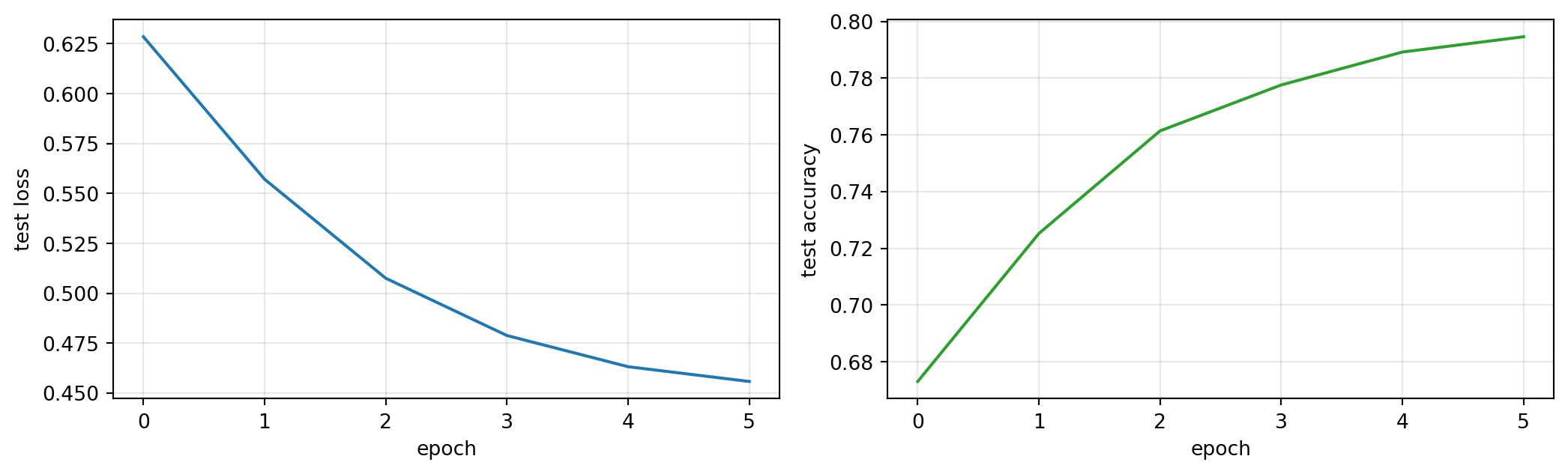
epoch 0  test loss 0.6285  test acc 0.6730
epoch 1  test loss 0.5571  test acc 0.7252
epoch 2  test loss 0.5075  test acc 0.7614
epoch 3  test loss 0.4788  test acc 0.7776
epoch 4  test loss 0.4632  test acc 0.7892
epoch 5  test loss 0.4558  test acc 0.7946

학습 시간 5초

fig, axes = plt.subplots(1, 2, figsize=(11, 3.4))
axes[0].plot(hist['loss']); axes[0].set_ylabel('test loss')
axes[1].plot(hist['acc'], color='C2'); axes[1].set_ylabel('test accuracy')
for ax in axes:
    ax.set_xlabel('epoch'); ax.grid(alpha=0.3)
plt.tight_layout(); plt.show()

6-5-5. 직접 문장을 넣어 본다

def predict(sentences):
    e = tok(sentences, padding=True, truncation=True, max_length=MAX_LEN, return_tensors='pt')
    model.eval()
    with torch.no_grad():
        p = model(e['input_ids'], e['attention_mask']).softmax(1)
    for s_, prob in zip(sentences, p):
        tag = '긍정' if prob[1] > 0.5 else '부정'
        print(f'{tag}  ({prob[1]:.3f})  {s_}')

predict([
    '연기도 좋고 스토리도 탄탄하다',
    '시간이 아깝다 최악',
    '기대했는데 그냥 그랬다',
    '눈물이 났다 정말 감동적이었다',
])

긍정  (0.802)  연기도 좋고 스토리도 탄탄하다
부정  (0.000)  시간이 아깝다 최악
부정  (0.055)  기대했는데 그냥 그랬다
긍정  (0.982)  눈물이 났다 정말 감동적이었다

이 모형이 못 하는 것

단어 순서를 전혀 보지 않는다. 마스크 평균은 토큰을 그냥 다 더해 나눌 뿐이라 “재미없지 않다”와 “재미있지 않다”를 구별할 방법이 없다.

\[\text{평균은 순서를 지운다}\]

다음 주에 토큰끼리 서로를 보게 만드는 어텐션으로 이 한계를 넘는다.

직접 해보기 ③ — 임베딩 차원을 바꿔 보기

d 를 16, 64, 256 으로 바꿔 학습시키고 파라미터 수와 정확도를 비교하시오.

def train_once(d, epochs=6):
    torch.manual_seed(42)
    m = SentimentNet(tok.vocab_size, d=d)
    ...                          # ← 위 6-5-4의 루프를 옮겨 오세요
    return sum(p.numel() for p in m.parameters()), acc

for d in [16, 64, 256]:
    ...